How AMM Algorithms Set Prices: A Simple Guide to DEX Math

Imagine walking into a grocery store where there is no cashier. Instead of scanning items and paying a human, you drop your groceries on a counter that automatically calculates the total based on how many other people have bought those same items today. That sounds chaotic, right? Yet, this is exactly how Automated Market Makers (AMMs) work in the world of decentralized finance.
If you have ever swapped tokens on Uniswap or Curve, you have interacted with an algorithm, not a person. These protocols replaced the traditional order book-where buyers and sellers match prices-with mathematical formulas that set prices instantly. But how does code decide what an asset is worth without a central authority?
The Core Mechanism: Liquidity Pools and Invariants
To understand how prices are set, you first need to understand where the money lives. In a centralized exchange like Coinbase, your trade matches against another person’s order. In a decentralized exchange (DEX), you trade against a liquidity pool. This is a smart contract holding two or more tokens, funded by users called liquidity providers (LPs).
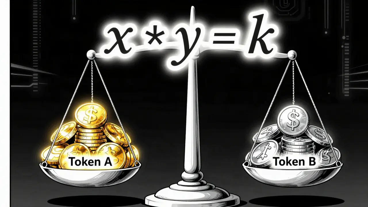
The price isn't fixed. It floats based on the ratio of assets in the pool. If there is more Token A than Token B in the pool, Token A becomes cheaper to buy because it is more abundant relative to demand. The algorithm enforces a rule called an invariant. An invariant is a mathematical value that must remain constant after every trade. Think of it as a balance scale. When you add weight to one side (buying tokens), you must remove weight from the other side (paying with other tokens) to keep the scale balanced according to the specific formula used.
This system allows for continuous trading 24/7 without needing a buyer and seller to be online at the exact same time. You are essentially borrowing from the pool, and the algorithm charges you a fee that goes to the LPs as compensation for their risk.
The Constant Product Formula: x * y = k
The most famous AMM model is the constant product formula, popularized by Uniswap V1 and V2. The formula looks simple: x * y = k.
- x: The amount of Token A in the pool.
- y: The amount of Token B in the pool.
- k: The constant value that cannot change.
Let’s look at a concrete example. Imagine a pool with 100 ETH and 200,000 USDC. The constant k is 20,000,000 (100 * 200,000). If you want to buy 10 ETH, you are increasing x to 110. To keep k at 20,000,000, the algorithm calculates that y must become approximately 181,818 USDC (20,000,000 / 110). This means you must pay about 18,182 USDC to get those 10 ETH.
The effective price per ETH for this trade is roughly 1,818 USDC. Notice that the initial price was 2,000 USDC per ETH (200,000 / 100). By buying a large chunk, you pushed the price up. This phenomenon is called slippage. The larger your trade relative to the pool size, the higher the slippage, and the worse the price you get. This protects LPs from being drained by large traders but can be costly for whales.
Beyond Constant Product: Weighted and Stable Swaps
While Uniswap’s model works well for volatile pairs like ETH/USDC, it fails miserably for stablecoins. If you try to swap USDT for USDC using the constant product formula, you will experience unnecessary slippage because these assets should always be worth $1. Enter different algorithms designed for specific use cases.
| Algorithm Type | Key Protocol Example | Best Use Case | Slippage Characteristic |
|---|---|---|---|
Constant Product (x*y=k) |
Uniswap V2 | Volatile assets (ETH/USDC) | High slippage for large trades |
| Weighted Geometric Mean | Balancer | Multi-token portfolios (e.g., 80% ETH, 20% DAI) | Customizable based on weights |
| StableSwap (Hybrid) | Curve Finance | Stablecoins (USDC/USDT) or pegged assets | Extremely low slippage near peg |
| Concentrated Liquidity | Uniswap V3 | Capital efficiency for LPs | Variable; depends on range selection |
Balancer uses a geometric mean formula that allows pools with more than two tokens and customizable weights. For instance, you can create a pool that is 80% ETH and 20% DAI. The algorithm adjusts prices to maintain this 80/20 ratio. If someone buys too much ETH, the price rises sharply to discourage further buying and restore balance. This is useful for investors who want to automate portfolio rebalancing.
Curve Finance revolutionized stablecoin trading with its StableSwap algorithm. It combines elements of constant sum (which has zero slippage but is vulnerable to arbitrage) and constant product. The result is a curve that is very flat near the 1:1 peg, meaning you can swap thousands of dollars of USDC for USDT with almost zero slippage. However, if the price deviates significantly from the peg (like during the UST crash in 2022), the curve steepens dramatically to protect LPs. Curve V2 added dynamic fees that adjust based on volatility, ensuring LPs earn more when the market is risky.
Concentrated Liquidity: Changing the Game
In May 2021, Uniswap V3 introduced concentrated liquidity. In previous versions, liquidity was spread across all possible prices, from $0 to infinity. Most of that capital was useless because ETH rarely trades at $1 or $10,000.
V3 allows liquidity providers to specify a price range, say $1,800 to $2,200. Your capital is only active within this band. This concentrates your liquidity, making it much more efficient. According to Uniswap Labs, this can improve capital efficiency by up to 4,000x compared to V2. For traders, this means deeper liquidity and lower slippage at current market prices. For LPs, it means higher fees earned on the same amount of capital.
However, this comes with a catch: impermanent loss. If ETH drops to $1,500, your liquidity stops earning fees because it is outside your range. You are left holding only ETH, which has lost value, while the USDC part of your position was sold at higher prices. Managing these ranges requires active monitoring or automated tools like Gamma.xyz.

Real-World Friction: Slippage and MEV
Even with sophisticated algorithms, trading on AMMs is not frictionless. Two major factors affect the final price you pay: slippage and Maximal Extractable Value (MEV).
Slippage is inherent to the math. As explained earlier, large trades move the price. Research by Georgios Konstantopoulos shows that on a standard Uniswap pool, a trade causing just 1% price impact requires only 0.33% of the total liquidity. This sensitivity means that deep liquidity is essential for healthy markets.
MEV is a darker side of blockchain economics. Because transactions sit in a mempool before being confirmed, bots can see your pending large swap. They might front-run your trade (buying before you to push the price up) and then back-run it (selling after you). This sandwich attack extracts profit from your trade, effectively increasing your slippage. EigenPhi reported that MEV cost users over $1.2 billion annually in 2023. While new solutions like TWAMM (Time-Weighted AMM) split large orders over time to hide intent, MEV remains a significant challenge for retail traders executing large swaps.
The Future: Hooks and Hybrid Models
The AMM landscape is evolving rapidly. The upcoming Uniswap V4 proposes "hooks," allowing developers to customize the pricing logic for each pool. This could lead to specialized AMMs for NFTs, leveraged positions, or real-world assets. Projects like Ambient Finance are experimenting with concentrated liquidity that doesn't require manual range management, aiming for high efficiency without the operational headache.
As DeFi matures, we are seeing hybrid models that combine the best of both worlds. SyncSwap, for example, uses adaptive curve parameters to achieve ultra-low slippage on stablecoins while maintaining flexibility for volatile pairs. The goal is clear: make decentralized trading as efficient and cheap as centralized exchanges, without sacrificing control.
Why do I get a different price than the market rate on a DEX?
This is due to slippage. AMM algorithms adjust prices based on supply and demand within the pool. If you buy a large amount of a token, you deplete the available supply in the pool, causing the algorithm to raise the price for subsequent units. The larger your trade relative to the pool's liquidity, the higher the slippage.
What is the difference between Uniswap V2 and V3 pricing?
Uniswap V2 spreads liquidity across all possible prices, leading to lower capital efficiency. V3 introduces concentrated liquidity, allowing providers to allocate funds within specific price ranges. This makes V3 more efficient for traders (lower slippage at current prices) but more complex for liquidity providers who must manage their ranges actively.
Is Curve Finance better than Uniswap for stablecoins?
Yes, for stablecoins, Curve is generally superior. Its StableSwap algorithm is designed to minimize slippage for assets with similar values (pegged assets). Uniswap's constant product formula creates unnecessary slippage for stablecoin swaps because it treats them like volatile assets. Curve achieves near-zero slippage for small-to-medium stablecoin trades.
How do liquidity providers make money if the price changes?
Liquidity providers earn trading fees from every swap executed in the pool. These fees are distributed proportionally to their share of the pool. However, they face impermanent loss, which occurs when the price of the deposited tokens changes significantly compared to when they were deposited. The fees must outweigh this loss for the strategy to be profitable.
Can AMMs be manipulated?
Yes, primarily through MEV (Maximal Extractable Value). Bots can monitor pending transactions and insert their own trades before or after yours to profit from the price movement. Additionally, flash loans can be used to temporarily manipulate pool prices, though newer protocols implement safeguards like Time-Weighted Average Price (TWAP) oracles to mitigate this.